Euler's Method Visualizer
Almost every ODEs instructor, including myself, has dreaded teaching about Euler’s method. The lesson is a rough one — it is highly computational, and it can seem unimportant to students taking the class. In some ways the students are correct. As an applied mathematician, I can attest to the fact that we rarely use Euler’s method in practice. It is outdated, unstable for stiff equations, and does not offer the conservative qualities of other geometric integrators.
However, it is the first, simplest, and often only numerical method students encounter, and it serves an important pedagogical purpose for motivating further study in numerical analysis. This blog post highlights some code which can (hopefully) make this lesson better.
A Quick Review of Euler’s Method
Consider a one dimensional ODE
\[ \frac{dy}{dt}=f(y,t) \]with smooth enough data. Via a Taylor expansion at \(t_0\)
\[ y(t_0+h) = y(t_0) + hy'(t_0) + \frac{h^2}{2}y''(t_0) +O(h^3). \]Since \(y'(t) = f(y(t),t),\) setting \(y_0 = y(t_0)\), the forward Euler update rule is
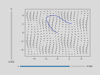
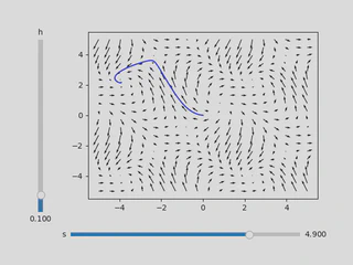
\[ y_0 = y(t_0), \quad t_n = t_{n-1}+h, \quad y_{n+1} = y_n+hf(y_n,t_n). \]Euler’s method easily generalizes to higher dimensional parameterized equations. Thanks to this, I created an Euler’s method visualizer for parameterized vector fields in two dimensions.
Example Vector Field
For the examples of this blog post, I will be visualizing the parameterized vector field
\[ \sin(x+y+s) \frac{\partial }{\partial x} + \left(\cos(x-s)+\sin\left( y\right) \right)\frac{\partial }{\partial y} \tag{1} \]with parameter \(s\). The initial condition is \((x_0,y_0) = (0,0)\).
Notice the difference between the two figures above: the vector field is the same, but the solutions diverge depending on the step size \(h\). This shows the sensitivity of Euler’s method to step size, especially near saddle points.
Parameter Sensitivity
Suppose we take \(s=4.8\) instead of \(s=4.9\):
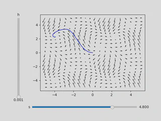
Although the vector fields are nearly identical, the fixed points of the approximated solutions are drastically different. This shows how small perturbations in a vector field can lead to large differences in the solution of an ODE.
We can quantify this by looking at the difference in vector magnitudes:
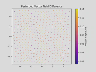
The maximum change is about 0.14, and the minimum change is about 0.02. Even these small differences affect the solution trajectory.
Since the system is autonomous, only vector angles matter. Here’s how the angle difference looks:
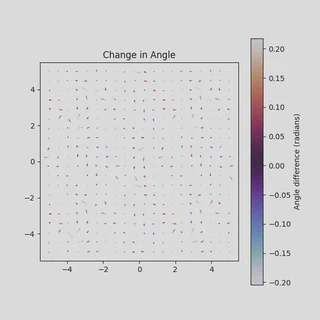
The maximum change in angle is around 0.2 radians — small, but significant enough to introduce instability in practice.
Further Questions
- How can we improve upon Euler’s method?
- How should one deal with an unstable system?
- Given a parameterized vector field, can we analyze its variation over a whole domain?
These questions connect to broader areas of numerical analysis and dynamical systems. I might expand on them in a future post. Until then, enjoy the vector field visualizer!
The GitHub repository is here.